使用python结合opencv占用栅格地图的实现(对数几率回归)(一)
占用栅格地图occupancy grid map 是将一张图片(width * height)用一些单元的小细胞格(cell)来进行拆分,然后可以使用贝叶斯的概率公式进行 “是0非1”的估算,在小细胞格子将概率值(0-1)乘以灰度值255 实现free和 occupancy的区分。如果某一个栅格的概率是0.5以上,乘以255后将使颜色变浅变白,则认为是free状态,反之,颜色越深即黑色说明是障碍物。
相关的数学推算可以参考《概率机器人》中的mapping章节。
但是本篇文章却使用对数几率回归的模型的实现建图。也是贝叶斯滤波的概率对数形式。

该篇讲述需要理解比较困难的有:
- 对数几率的定义:如果某事件发生的概率为Px ,则反例为1-Px,两者的比值 Px/(1-Px) 为几率odds.
对其求ln ,则为 ln Px/(1-Px) 称为对数几率。英文名称log odds ,对数几率的出现是为了预测真实结果的回归。是一种学习算法。
是一种用于分类的线性回归模型。


下图的推导公式再接下来的代码中即将用到

接下来使用diy的机器车rovi进行实验,rovi车三面有三个超声波雷达,用于测距和构建实时的栅格地图使用。rovi将数据保存成data.txt然后python读取
data.txt进行测试。

senseor_modle.py
如下
import cv2
import numpy as np
import os
import math
from mpl_toolkits.mplot3d import axes3d
import matplotlib.pyplot as plt

#####################################################################################################################################
# Sonar Model
# occmap = map array, Xr = Robot X coordinate, Yr = Robot Y coordinate, Rangle = Robot heading in degrees, SonarDist = Sonar reading in mm
# thickness = Object thickness in mm, Scale = float map scale
#
# Returns: Sonar_log - Array of log odds probabilities. This can be added to existing log odds occ map to update map with latest sonar data.
#          occ - Array of occupied points for scan matching
#####################################################################################################################################
def SonarModel(occmap, Xr, Yr, Rangle, SonarDist, thickness, scale):

    Sonar_mask = np.zeros((occmap.shape),np.uint8)
    Sonar_log = np.zeros((occmap.shape),np.single)
    robotpt = (Xr,Yr)

    thickness = int(thickness * scale)
    SonarDist = int(SonarDist * scale)

    cv2.ellipse(Sonar_mask,(int(Xr),int(Yr)),(SonarDist, SonarDist), Rangle, -15, 15, 255, -1) #Draw ellipse on to sonar mask

    pixelpoints = cv2.findNonZero(Sonar_mask) #Find all pixel points in sonar cone

    occ = np.empty((0,1,2),int)

    for x in pixelpoints:

        Ximg = x[0][0] # is a value x
        Yimg = x[0][1] #
        dist = np.linalg.norm(robotpt - x) #Find euclidean distance to all points in sonar cone from robot location

        theta = (math.degrees(math.atan2((Yimg-Yr),(Ximg-Xr)))) - Rangle #Find angle from robot location to each cell in pixelpoints

        if theta < -180:                                                 #Note:numpy and OpenCV X and Y reversed
            theta = theta + 360
        elif theta > 180:
            theta = theta - 360
        #正态分布的公式  sigma为5 位置参数u为角度theta
        sigma_t = 5
        A = 1 / (math.sqrt(2*math.pi*sigma_t))
        C = math.pow((theta/sigma_t),2)
        B = math.exp(-0.5*C)
        Ptheta = A*B

        Pdist = (SonarDist - dist/2)/SonarDist
        P = (Pdist*2)*Ptheta

        print dist,SonarDist,thickness
        if dist > SonarDist - thickness and dist < SonarDist + thickness: #occupied region
            Px = 0.5 + Ptheta
            logPx = math.log(Px/(1-Px))
            Sonar_log[Yimg][Ximg] = logPx
            #print logPx
            #occ = np.append(occ,[x],0)
        else: #free region
            Px = 0.5 - P
            logPx = math.log(Px/(1-Px))
            Sonar_log[Yimg][Ximg] = logPx

    return Sonar_log, occ

#####################################################################################################################################
# IR Model
# occmap = map array, Xr = Robot X coordinate, Yr = Robot Y coordinate, Rangle = Sensor heading in degrees, IRDist = IR reading in mm
# thickness = Object thickness in mm, Scale = float map scale
#
# Returns: IR_log - Array of log odds probabilities. This can be added to existing log odds occ map to update map with latest sonar data.
#          occ - Array of occupied points for scan matching
#####################################################################################################################################
def IRModel(occmap, Xr, Yr, Rangle, IRDist, thickness, scale):

    IR_mask = np.zeros((occmap.shape),np.uint8)
    IR_log = np.zeros((occmap.shape),np.single)

    if IRDist == 0:
        print 'IR Zero'
        return IR_log

    robotpt = (Xr,Yr)
    IR_Max = int(600 * scale)

    thickness = int(thickness * scale)
    IRDist = int(IRDist * scale)

    XIR = Xr + float((math.cos(math.radians(Rangle)) * IRDist))
    YIR = Yr + float((math.sin(math.radians(Rangle)) * IRDist))

    cv2.line(IR_mask, (int(Xr),int(Yr)), (int(XIR),int(YIR)), 255, 1)
    pixelpoints = cv2.findNonZero(IR_mask) #Find all pixel points in sonar cone

    occ = np.empty((0,1,2),int)

    for x in pixelpoints:
        Ximg = x[0][0]
        Yimg = x[0][1]
        dist = np.linalg.norm(robotpt - x) #Find euclidean distance to all points in sonar cone from robot location

        Pdist = (IRDist - (dist/2))/IRDist

        if dist > IRDist - thickness and dist < IRDist + thickness: #occupied region
            if IRDist < IR_Max: #Only update occupied region if IR reading is less than maximum.
                Px = 0.8
                logPx = math.log(Px/(1-Px))
                IR_log[Yimg][Ximg] = logPx
                #occ = np.append(occ,[x],0)
        else: #free region
            Px = 0.3#0.5 - (Pdist/3)
            logPx = math.log(Px/(1-Px))
            IR_log[Yimg][Ximg] = logPx

    return IR_log, occ

if __name__ == "__main__":

    Xr = float(50)
    Yr = float(50)

    scale = float(1)/100

    cv2.namedWindow("Sonar", cv2.WINDOW_NORMAL)
    cv2.resizeWindow("Sonar", 1000, 1000)
    cv2.waitKey(1)

    Map_log = np.full((100,100),0,np.single)

    #IR_log, occ = IRModel(Map_log, Xr, Yr, -45, 590, 100, scale)
    #Map_log = np.add(Map_log, IR_log)

    Sonar_log, occ = SonarModel(Map_log, Xr, Yr, -90, 4500, 100, scale)

    #Map_log = np.add(Map_log, Sonar_log)
    Map_log =cv2.add(Map_log, Sonar_log)
    #Map_P = 1 - (1/(1+(np.exp(Map_log))))
    #Disp_img = 1-Map_P

    Disp_img = (1/(1+(np.exp(Map_log))))
    cv2.imshow("Sonar", Disp_img)
    cv2.waitKey(1)

    #'''
    #Plot as matplotlib 3D plot
    fig = plt.figure()
    ax = fig.add_subplot(111, projection='3d')

    #plt.axis('off')
    #x = np.arange(0,100,1)
    #y = np.arange(0,100,1)
    #X, Y = np.meshgrid(x, y)
    #ax.plot_wireframe(X, Y, Map_P)
    #plt.show()
    #'''

    cv2.waitKey(0) #Leave window open

'''
Sonar_log = SonarModel(Map_log, Xr, Yr, -90, 6000, 100, scale)
Map_log = np.add(Map_log, Sonar_log)
Map_P = 1 - (1/(1+(np.exp(Map_log))))
Disp_img = 1-Map_P

cv2.imshow("Sonar", Disp_img)
cv2.waitKey(1)
'''
python sensormodel.py
测试效果如下图
 下一篇将介绍,上面的python代码如何使用 opencv c++ 实现,研究每个函数的替代性。